
Introduction to Evaluation Metrics for Data Classification
Author: Kamile Yagci
Theory
The evaluation metrics are used to measure the performance of data classification models. In this post, I will focus on binary classifcation, where predicted values are 1 (True) or 0 (False).
The binary classification model prediction has four possible labels: True Positive (TP), True Negative (TN), False Positive (FP) and False Negative (FN). We can visualize these labels in matrix form:
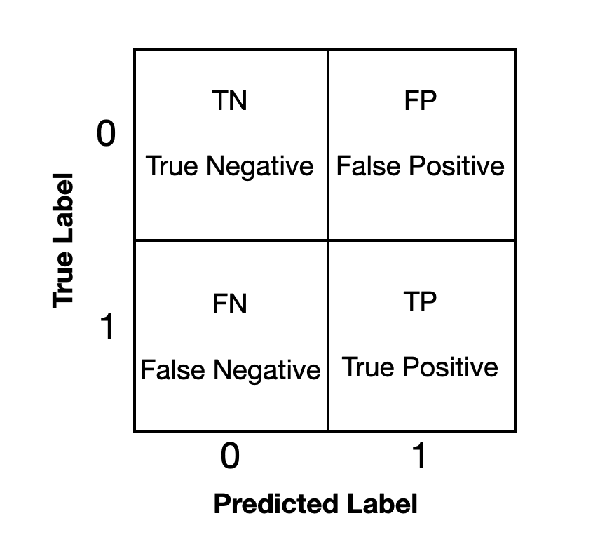
We calculate evaluation metrics using these labels. Here are the short description of the metrics:
1. Precision: What percentage of my predictions are true?
\[precision = \frac{\text{# of True Positives}}{\text{# of Predicted Positives}} = \frac{TP}{TP+FP}\]2. Recall: What percentage of the class I am interested is correctly identified by the model?
\[recall = \frac{\text{# of True Positives}}{\text{# of Total Actual Positives}} = \frac{TP}{TP + FN}\]3. Accuracy: What percentage of my predictions are correct
\[accuracy = \frac{\text{# of True Positives + # of True Negatives}}{\text{# of Total Observations}} = \frac{(TP + TN)}{(TP + TN + FP + FN)}\]4. f1-score: Harmonic Mean of Precision and Recall
\[f1 = 2 * \frac{Precision * Recall}{Precision + Recall}\]5. ROC-AUC: Area under the ROC Curve
ROC: Receiver Operating Characteristic curve: graphical plot that illustrates the true positive rate (TPR) against the false positive rate (FPR).
- TPR = # of true positives / # of total actual positives = TP/(TP+FN) = ‘recall’
- FPR = # of false positives / # of total actual positives = FP/(TP+FN)
Which metric score is best to measure the model performance?
It all depends on the purpose of the study.
Let’s answer this question with examples:
Example 1 - High Blood Pressure
My goal is make a prediction if a person will have high blood pressure problem in future. The data provided contains some physical properties and some medical test results of the patient.
The metric I most care is the ‘recall’, since we want to identify as many as at-risk patients. However, the ‘precision’ is inversely proportional to recall. If I put loose threshold for labeling at-risk patients, then it is very likely that you will have many false positives besides true positives. If I put sctrict threshold, then I will miss many positive cases, wheras the precision is high.
For medical studies like this one, it is better to keep a loose threshold in identification, and keep the ‘recall’ at high value. Moreover, I would also keep an eye on ‘f1-score’, harmonic mean of precision and recall, to make sure precision is not very low.
Example 2 - Beauty Product Sales
The beauty company has a new product and plan to introduce and sell it to customers via phone calls. The company has a database of past customer purchases. My goal is make a list of the customers who will most likely to purchase it.
Since there are limited number of phone operators, my list should have a high precision. For high efficieny of the call process, the percentage of customers who buys the product after the phone calls should be high. Therefore, the metric I focus on is ‘precision’. Again, I would make sure that f1-score is not low.
Accuracy and Imbalanced Datasets
The accuracy is a commonly used to check the performance classification models. It is the default scoring for many SciKit-Learn Classifiers. It works well when dataset has balanced class distribution; about 50% True (1) and 50% False (0) values.
However, the accuracy score may be misleading when the dataset is imbalanced; the True values are significantly larger or smaller than the False values.
I will explain the inbalanced datasets more detailed and show the solution in next section.
Evaluation Metrics on SyriaTel Customer Churn Study
The SyriaTel, the telecommunication company, wants to predict whether a customer will (“soon”) stop doing business with them.
Question: Choose a model which will best identify the customers who will stop doing business with SyriaTel
The target variable for this study is ‘churn’. The rest of the variables in the dataset will be predictors.
‘churn’: activity of customers leaving the company and discarding the services offered
Load and pre-process Data
# Import base libraries
import pandas as pd
import numpy as np

import matplotlib.pyplot as plt
%matplotlib inline
import seaborn as sns

import warnings
warnings.filterwarnings('ignore')
# Load and Clean data
df = pd.read_csv('bigml_59c28831336c6604c800002a.csv')

df = df.drop('phone number', axis=1)

df['international plan'] = df['international plan'].map({'yes':1 ,'no':0})
df['voice mail plan'] = df['voice mail plan'].map({'yes':1 ,'no':0})
df['churn'] = df['churn'].map({True:1 ,False:0})

df = df.astype({'international plan': 'object'})
df = df.astype({'voice mail plan': 'object'})
df = df.astype({'area code': 'object'})

#df.head()
df.info()
<class 'pandas.core.frame.DataFrame'>
RangeIndex: 3333 entries, 0 to 3332
Data columns (total 20 columns):
 #   Column                  Non-Null Count  Dtype
---  ------                  --------------  -----
 0   state                   3333 non-null   object
 1   account length          3333 non-null   int64
 2   area code               3333 non-null   object
 3   international plan      3333 non-null   object
 4   voice mail plan         3333 non-null   object
 5   number vmail messages   3333 non-null   int64
 6   total day minutes       3333 non-null   float64
 7   total day calls         3333 non-null   int64
 8   total day charge        3333 non-null   float64
 9   total eve minutes       3333 non-null   float64
 10  total eve calls         3333 non-null   int64
 11  total eve charge        3333 non-null   float64
 12  total night minutes     3333 non-null   float64
 13  total night calls       3333 non-null   int64
 14  total night charge      3333 non-null   float64
 15  total intl minutes      3333 non-null   float64
 16  total intl calls        3333 non-null   int64
 17  total intl charge       3333 non-null   float64
 18  customer service calls  3333 non-null   int64
 19  churn                   3333 non-null   int64
dtypes: float64(8), int64(8), object(4)
memory usage: 520.9+ KB
# Assign target and predictor
y = df['churn']
X = df.drop('churn', axis=1)

# Create dummy variables
X = pd.get_dummies(X)
# Sepearate data into train and test splist
from sklearn.model_selection import train_test_split

X_train, X_test, y_train, y_test = train_test_split(X, y, random_state=42)

print('X_train shape = ', X_train.shape)
print('y_train shape = ', y_train.shape)
print('X_test shape = ', X_test.shape)
print('y_test shape = ', y_test.shape)
X_train shape =  (2499, 73)
y_train shape =  (2499,)
X_test shape =  (834, 73)
y_test shape =  (834,)
# Scale/Normalize the predictor variables
from sklearn.preprocessing import StandardScaler

scaler = StandardScaler()
X_train_scaled = scaler.fit_transform(X_train)
X_test_scaled = scaler.transform(X_test)

# Convert to Dataframe
X_train_scaled = pd.DataFrame(X_train_scaled, columns=X_train.columns)
X_test_scaled = pd.DataFrame(X_test_scaled, columns=X_test.columns)
#X_train_scaled.head()
Logistic Regression Model
I start with Logistic Regression. I instantiate the model with default parameters and fit on training data.
Then I check the evaluation metrics both for training and testing data.The Scikit-Learn classification_report function lists the evaluation metric values for each class; churn=0 and churn=1.
from sklearn.linear_model import LogisticRegression
from sklearn.metrics import confusion_matrix, plot_confusion_matrix, classification_report

logreg = LogisticRegression(random_state=42)
logreg.fit(X_train_scaled, y_train)

print('Training Data:\n', classification_report(y_train, logreg.predict(X_train_scaled)))
print('Testing Data:\n', classification_report(y_test, logreg.predict(X_test_scaled)))
Training Data:
               precision    recall  f1-score   support

           0       0.89      0.97      0.93      2141
           1       0.64      0.27      0.37       358

    accuracy                           0.87      2499
   macro avg       0.76      0.62      0.65      2499
weighted avg       0.85      0.87      0.85      2499

Testing Data:
               precision    recall  f1-score   support

           0       0.88      0.97      0.92       709
           1       0.56      0.22      0.32       125

    accuracy                           0.86       834
   macro avg       0.72      0.60      0.62       834
weighted avg       0.83      0.86      0.83       834
Evaluation metrics for the test data tells that:
- The model identified the 22% of the actual customers correctly.
- 56% of the predicted churn customers are actual churn.
- f1-score is 32%.
- The precision - recall - f1 scores are low (for churn=1), so the model prediction performance is not good.
- The accuracy of the predictions is 85%. The accuracy score is high, but misleading. It is caused by the imbalanced dataset.
- The metrics look similar for both training and testing data, just training is a bit better; so slight overfitting.
Let’s check the class distributions of the whole data (train + test):
print('Original whole data class distribution:')
print(y.value_counts())
print('Original whole data class distribution, normalized:')
print(y.value_counts(normalize=True))
Original whole data class distribution:
0    2850
1     483
Name: churn, dtype: int64
Original whole data class distribution, normalized:
0    0.855086
1    0.144914
Name: churn, dtype: float64
According to the dataset, 85.5% of the customers do continue with SyriaTel and 14.5% of customers stop business. If we make a prediction saying all customers will continue business, then we will have about 85.5% accuracy. This explains the high accuracy score of the model, despite the other low metric values.
I use SMOTE to create a synthetic training sample to take care of imbalance. After the resampling, the value counts in each class, in training data sample, becomes equal.
# Import SMOTE, resample
from imblearn.over_sampling import SMOTE

smote = SMOTE()
X_train_scaled_resampled, y_train_resampled = smote.fit_resample(X_train_scaled, y_train)

print('Original training data class distribution:')
print(y_train.value_counts())
print('Synthetic training data class distribution:')
print(y_train_resampled.value_counts())
Original training data class distribution:
0    2141
1     358
Name: churn, dtype: int64
Synthetic training data class distribution:
1    2141
0    2141
Name: churn, dtype: int64
# New model after resampling
logreg = LogisticRegression(random_state=42)
logreg.fit(X_train_scaled_resampled, y_train_resampled)

print('Training Data:\n', classification_report(y_train_resampled, logreg.predict(X_train_scaled_resampled)))
print('Testing Data:\n', classification_report(y_test, logreg.predict(X_test_scaled)))
Training Data:
               precision    recall  f1-score   support

           0       0.80      0.78      0.79      2141
           1       0.79      0.80      0.80      2141

    accuracy                           0.79      4282
   macro avg       0.79      0.79      0.79      4282
weighted avg       0.79      0.79      0.79      4282

Testing Data:
               precision    recall  f1-score   support

           0       0.95      0.79      0.86       709
           1       0.39      0.77      0.51       125

    accuracy                           0.78       834
   macro avg       0.67      0.78      0.69       834
weighted avg       0.87      0.78      0.81       834
Evaluation metrics for the test data tells that:
- The model identifies the 77% of the actual real customers correctly.
- 39% of the predicted churn customers are actual churn.
- f1-score is 51%.
- The recall and f1-score are improved, which is good for our model.
- The accuracy of the predictions is 78%. It is a bit worse than random guessing.
- There is overfitting.
Decision Tress
# Import, Instantiate, fit DecisionTreeClassifier,
from sklearn.tree import DecisionTreeClassifier

dt = DecisionTreeClassifier(random_state=42)
#dt.fit(X_train_scaled, y_train)
dt.fit(X_train_scaled_resampled, y_train_resampled)

print('Training Data:\n', classification_report(y_train_resampled, dt.predict(X_train_scaled_resampled)))
print('Testing Data:\n', classification_report(y_test, dt.predict(X_test_scaled)))
Training Data:
               precision    recall  f1-score   support

           0       1.00      1.00      1.00      2141
           1       1.00      1.00      1.00      2141

    accuracy                           1.00      4282
   macro avg       1.00      1.00      1.00      4282
weighted avg       1.00      1.00      1.00      4282

Testing Data:
               precision    recall  f1-score   support

           0       0.94      0.91      0.92       709
           1       0.56      0.69      0.62       125

    accuracy                           0.87       834
   macro avg       0.75      0.80      0.77       834
weighted avg       0.89      0.87      0.88       834
Evaluation metrics for the test data tells that:
- The model identifies the 69% of the actual real customers correctly.
- 56% of the predicted churn customers are actual churn.
- f1-score is 2%.
- The accuracy of the predictions is 87%. It is slightly better than random guessing.
- Overfitting is observed.
XGBoost
# Import, Instantiate, fit XGBClassifier
from xgboost import XGBClassifier
import xgboost as xgb

xgb = XGBClassifier(random_state=42, eval_metric='logloss') #'logloss' is default, but specified to stop warning
#xgb.fit(X_train_scaled, y_train)
xgb.fit(X_train_scaled_resampled, y_train_resampled)

print('Training Data:\n', classification_report(y_train_resampled, xgb.predict(X_train_scaled_resampled)))
print('Testing Data:\n', classification_report(y_test, xgb.predict(X_test_scaled)))
Training Data:
               precision    recall  f1-score   support

           0       1.00      1.00      1.00      2141
           1       1.00      1.00      1.00      2141

    accuracy                           1.00      4282
   macro avg       1.00      1.00      1.00      4282
weighted avg       1.00      1.00      1.00      4282

Testing Data:
               precision    recall  f1-score   support

           0       0.96      0.98      0.97       709
           1       0.88      0.77      0.82       125

    accuracy                           0.95       834
   macro avg       0.92      0.87      0.90       834
weighted avg       0.95      0.95      0.95       834
Evaluation metrics for the test data tells that:
- The model identifies the 77% of the actual real customers correctly.
- 88% of the predicted churn customers are actual churn.
- f1-score is 82%.
- The accuracy of the predictions is 95%. It is better than random guessing.
- There is overfitting.
Model Comparison
At this section, I compare the classification models to choose the best one to identify the customers who will study doing business with SyriaTel .
I look evaluation metrics like precision, recall, accuracy and f1.
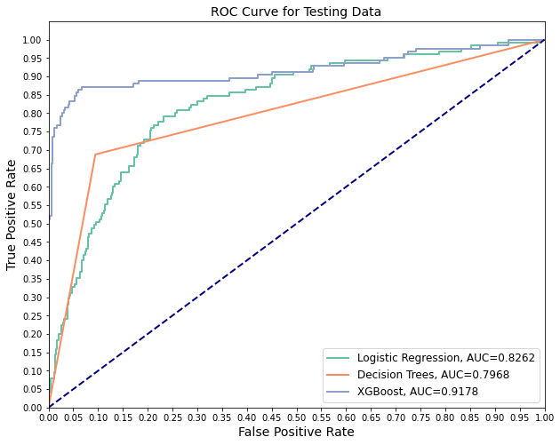
I also plot ROC curves and calculate AUC for each model.
from sklearn.metrics import roc_curve, auc
from sklearn.metrics import precision_score, recall_score, accuracy_score, f1_score

model_list = [logreg, dt, xgb]
model_names = ['Logistic Regression', 'Decision Trees', 'XGBoost']

def model_scores(dataset_type, X_scaled, y_true):
    """
    dataset_type = 'Testing' or 'Training'
    X_scaled = X_test_scaled or X_train_scaled
    y_true = y_train or y_test

    """
    colors = sns.color_palette('Set2')
    plt.figure(figsize=(10, 8))

    model_scores_list = []

    for n, clf in enumerate(model_list):
        #print(n)

        clf.fit(X_train_scaled_resampled, y_train_resampled)

        y_pred = clf.predict(X_scaled)

        #y_score = clf.decision_function(X_scaled)
        y_prob = clf.predict_proba(X_scaled) #Probability estimates for each class
        fpr, tpr, thresholds = roc_curve(y_true, y_prob[:,1])
        auc_score = auc(fpr, tpr)
        plt.plot(fpr, tpr, color=colors[n], lw=2, label=f'{model_names[n]}, AUC={round(auc_score, 4)}')

        fit_scores = {'model': model_names[n],
                        'precision': precision_score(y_true, y_pred),
                        'recall': recall_score(y_true, y_pred),
                        'accuracy': accuracy_score(y_true, y_pred),
                        'f1': f1_score(y_true, y_pred),
                        'auc': auc_score
                       }

        model_scores_list.append(fit_scores)

    plt.plot([0, 1], [0, 1], color='navy', lw=2, linestyle='--')
    plt.xlim([0.0, 1.0])
    plt.ylim([0.0, 1.05])
    plt.yticks([i/20.0 for i in range(21)])
    plt.xticks([i/20.0 for i in range(21)])
    plt.xlabel('False Positive Rate', fontsize=14)
    plt.ylabel('True Positive Rate', fontsize=14)
    plt.title(f'ROC Curve for {dataset_type} Data', fontsize=14)
    plt.legend(loc='lower right', fontsize=12)
    #plt.show()
    plt.savefig(f'images/ROC_Curve_{dataset_type}.png')


    model_scores_df = pd.DataFrame(model_scores_list)
    model_scores_df = model_scores_df.set_index('model')
    print(model_scores_df)

    #return model_scores_df
    return None
model_scores('Testing', X_test_scaled, y_test)
                     precision  recall  accuracy        f1       auc
model
Logistic Regression   0.387097   0.768  0.782974  0.514745  0.826212
Decision Trees        0.562092   0.688  0.872902  0.618705  0.796750
XGBoost               0.880734   0.768  0.949640  0.820513  0.917822
Interpret
Which model is best on identinfying churn customers?
According to the results, I choose the XGBoost classifier as best model.
The ‘f1-score’ is significantly larger than other models, even though the ‘recall value is slighty smaller. Moreover, the AUC is highest for XGBoost.
The scikit-learn confusion_matrix displays the true and predicted labels.
# Confusion matrix for test data
plot_confusion_matrix(xgb, X_test_scaled, y_test)
plt.savefig('images/confusion_matrix_XGB.png')
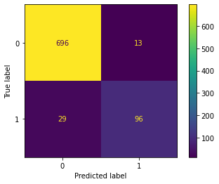
- XGBoost model identification statistics on test data:
- Number of true positives: 96
- Number of true negatives: 696
- Number of false positives: 13
- Number of false negatives: 29
- The final model identifies 96 out of 125 churn customers correctly (77% recall).
- 96 out of 109 predicted churn customers are real churn (88% precision).
Further ….
I used the default paremeters of Classifiers when instantiating models in this blog post. However, model performance can be improved by parameter tuning with GridSearchCV. It determines the best parameter combination for the given parameter grid list.
Moreover, overfitting is observed in all models. It needs to be addressed.
In my SyriaTel Churn Customer Study, I chose to use f1-score for parameter tuning. The parameter tuning increased the model performance of XGBoot Classifier. I also decreased the overfitting with controllling the max_depth parameter. Since the main goal of this blog post is introducing the evaluation metrics, I haven’t inlcuded these components of my project here.