
Basics of Linear Regression with Scikit-Learn
Author: Kamile Yagci
In this blog, I go over the basics of Linear Regression model using Scikit-Learn library.
Content:
- Data
- Theory of Linear Regression
- Data Splitting into Training and Testing subsets (train_test_split)
- Linear Regression Fit and Model Validation (LinearRegression)
- Baseline Linear Regression - one predictor
- Multiple Linear Regression - Multiple predictor
- Cross Validation (cross_val_score, cross_validate, ShuffleSplit)
#Import Libraries
import pandas as pd
import matplotlib.pyplot as plt
%matplotlib inline
import seaborn as sns
import numpy as np
Explore Data
I will use King County House Sales data. My goal is predict the House Sale price by using Linear Regression.
At first, I will take a brief look at data.
#Load data file, get general info, and check for missing values
df = pd.read_csv('data/kc_house_data.csv')
df.info()
<class 'pandas.core.frame.DataFrame'>
RangeIndex: 21597 entries, 0 to 21596
Data columns (total 21 columns):
 #   Column         Non-Null Count  Dtype
---  ------         --------------  -----
 0   id             21597 non-null  int64
 1   date           21597 non-null  object
 2   price          21597 non-null  float64
 3   bedrooms       21597 non-null  int64
 4   bathrooms      21597 non-null  float64
 5   sqft_living    21597 non-null  int64
 6   sqft_lot       21597 non-null  int64
 7   floors         21597 non-null  float64
 8   waterfront     19221 non-null  float64
 9   view           21534 non-null  float64
 10  condition      21597 non-null  int64
 11  grade          21597 non-null  int64
 12  sqft_above     21597 non-null  int64
 13  sqft_basement  21597 non-null  object
 14  yr_built       21597 non-null  int64
 15  yr_renovated   17755 non-null  float64
 16  zipcode        21597 non-null  int64
 17  lat            21597 non-null  float64
 18  long           21597 non-null  float64
 19  sqft_living15  21597 non-null  int64
 20  sqft_lot15     21597 non-null  int64
dtypes: float64(8), int64(11), object(2)
memory usage: 3.5+ MB
# List null values
df.isnull().sum()
id                  0
date                0
price               0
bedrooms            0
bathrooms           0
sqft_living         0
sqft_lot            0
floors              0
waterfront       2376
view               63
condition           0
grade               0
sqft_above          0
sqft_basement       0
yr_built            0
yr_renovated     3842
zipcode             0
lat                 0
long                0
sqft_living15       0
sqft_lot15          0
dtype: int64
# A bit of data cleaning
df['waterfront'].fillna(0., inplace=True)
# Correlation heatmap
plt.figure(figsize=(12,10))
sns.heatmap(df.corr(), center=0);
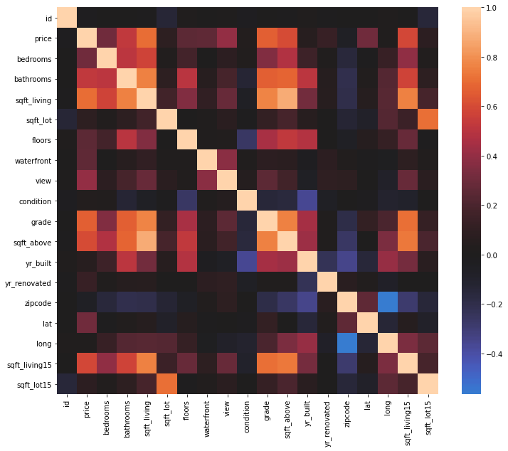
In this study, my target variable is ‘price’. The rest of the variables are ‘predictors’. We can use one or multiple predictors in modeling.
The correlation heatmap visualize the correlation between the variables and help us to choose good predictors.
Based on the above heatmap, there is a good correlation between ‘price’ and ‘sqft_living’.
Theory of Linear Regression
Linear equation with one independent variable is
y = mx + b
where
- x is the independent variable,
- y is dependent varaible,
- m is slope and
- b is y-intercept.
In our model:
- dependent variable is target variable ‘price’ (y)
- independent variable is the predictor such as ‘sqft_living’ (X)
When linear fit is applied to the data that consists of X and y, it determines the line of best fit. The slope and y-intercept of this line are the parameters of the model.
In multiple linear regression, we use more than one predictors:
y = b + m1x1 + m2x2 + m3x3 + …..
where X = [x1, x2, x3, …]
Splitting Data into Training and Testing subsets (train_test_split)
After modeling the data, we need to test it. However, we cannot use the same set of data for both modeling and testing. There is a possibility that data is overfitted. The overfitted model will work well for the dataset in which the model is created, but it will not give good results with another set of data.
Therefore, we split our data into two subsets: training and testing. We use the training data for modeling and the testing data for comparing the predictions with the actual data.
The scikit-Learn library has a function for splitting the data randomly:
sklearn.model_selection.train_test_split(*arrays, test_size=None, train_size=None, random_state=None, shuffle=True, stratify=None)
* Input: X and y
* Output: Lists of X_train, X_test, y_train, y_test
The default test_size = 0.25, so the train_size is 0.75. It is recommended to allocate at least half of the data for training.
# Import train_test_split
from sklearn.model_selection import train_test_split
# Assign X and y
y = df['price'] # Dataseries for Target, dependent variable
X = df.drop('price', axis=1) # Dataframe for Predictors, independent variables
# Seperate data into training and testing splits
X_train, X_test, y_train, y_test = train_test_split(X, y, random_state=0)

print(f"X_train is a DataFrame with {X_train.shape[0]} rows and {X_train.shape[1]} columns")
print(f"y_train is a Series with {y_train.shape[0]} values")
X_train is a DataFrame with 16197 rows and 20 columns
y_train is a Series with 16197 values
Linear Regression Fit and Model Validation (LinearRegression)
The scikit-Learn class for linear regression:
class sklearn.linear_model.LinearRegression(*, fit_intercept=True, normalize='deprecated', copy_X=True, n_jobs=None, positive=False)
* Input: X and y
* Output: Linear regression model
* Attributes:
    * _coef: coefficient / slope of the line-of-best-fit (for each predictor)
    * intercept_: y-intercept of the line-of-best-fit
* Methods:
    * fit(X, y): fit linear model
    * predict(X): predict y using the model
    * score(X, y): return R squared
P.S. Not all attributes and methods of LinearRegression() are listed here.
#Import LinearRegression
from sklearn.linear_model import LinearRegression
Baseline Linear Regression - one predictor
Let’s start modeling data with one predictor. * X: ‘sqft_living’ * y: ‘price’
We will only use training data for modeling.
# Apply LinearRegression on Training Data
baseline_model = LinearRegression()

X_train_sqft = X_train[['sqft_living']]  # Dataframe with predictor columns, training data

regline = baseline_model.fit(X_train_sqft, y_train) # fitted model

print("Slope:", regline.coef_) # print cefficient/slope
print("y-intercept:", regline.intercept_) # print y-intercept
print("R squared for Training:", regline.score(X_train_sqft, y_train)) # print R squared
Slope: [285.58593563]
y-intercept: -53321.493253810564
R squared for Training: 0.4951005996564265
The above code fitted the data, created the model and printed out the results.
The slope and y-intercept values describes the line-of-best-fit.
The R squared score is the coefficient of determination. It tells us how good the Linear Regression fit is. The R squared ranges from 0 to 1. The higher score means a better fit.
Model Validation
Our model is based on Training data. How will it perform on Testing data?
We will answer this questions by applying our model on test data. It will calculate the R squared score; how close our line-of-best-fit to the testing data.
# Model validation
X_test_sqft = X_test[['sqft_living']] # Dataframe with predictor column, testing data

print("R squared for Training:", regline.score(X_train_sqft, y_train))
print("R squared for Testing:", regline.score(X_test_sqft, y_test))
R squared for Training: 0.4951005996564265
R squared for Testing: 0.48322207729033984
R squared score for training and testing data is close. We can conclude that the model works well on testing data.
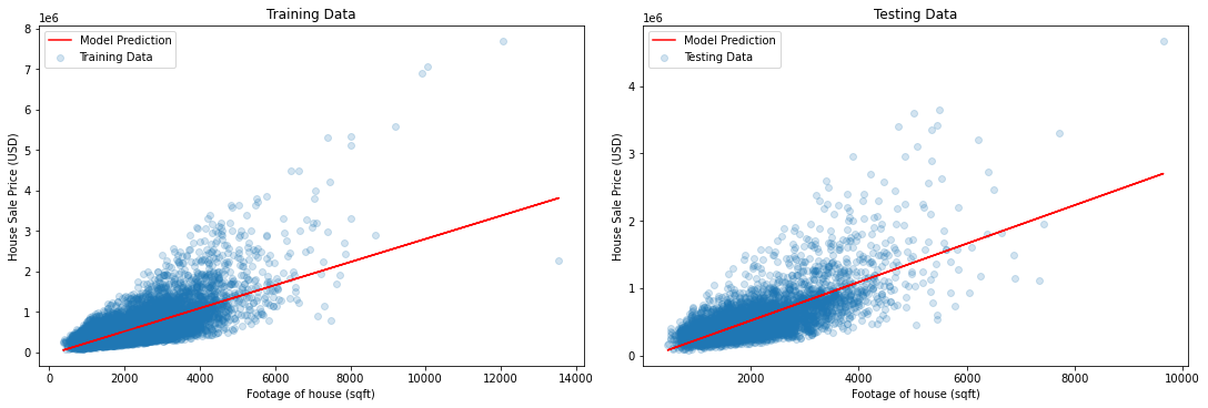
Let’s do some visualization to see how good our Linear Regression model, line-of-best fit.
# Visualization

y_train_hat = baseline_model.predict(X_train_sqft)  # model predictions for target, training data
y_test_hat = baseline_model.predict(X_test_sqft) # model predictions for target, testing data

fig, (ax1, ax2) = plt.subplots(1, 2, figsize=(15, 5), constrained_layout=True)

ax1.scatter(X_train_sqft, y_train, label='Training Data', alpha=0.2)
ax1.plot(X_train_sqft, y_train_hat, color='red', label='Model Prediction')
ax1.set_xlabel("Footage of house (sqft)")
ax1.set_ylabel("House Sale Price (USD)")
ax1.set_title("Training Data")
ax1.legend()

ax2.scatter(X_test_sqft, y_test, label='Testing Data', alpha=0.2)
ax2.plot(X_test_sqft, y_test_hat, color='red', label='Model Prediction')
ax2.set_xlabel("Footage of house (sqft)")
ax2.set_ylabel("House Sale Price (USD)")
ax2.set_title("Testing Data")
ax2.legend()
<matplotlib.legend.Legend at 0x7fae0f99f2b0>
Multiple Linear Regression - Multiple predictor
Instead of using one predictor, we can use multiple predictors to model our data. We call this Multiple Linear Regression.
- X: [‘sqft_living’, ‘waterfront’, ‘year_built’]
- y: ‘price’
multi_model = LinearRegression()

pred = ['sqft_living', 'waterfront', 'yr_built'] # Define predictors

X_train_multi = X_train[pred]
X_test_multi = X_test[pred]

regline = multi_model.fit(X_train[pred], y_train)

print('Final model predictors:', pred)
print("Slope:", regline.coef_) # print coefficients for each predictor
print("y-intercept:", regline.intercept_) # print y-intercept
print("R squared for Training:", regline.score(X_train_multi, y_train))
print("R squared for Testing:", regline.score(X_test_multi, y_test))
Final model predictors: ['sqft_living', 'waterfront', 'yr_built']
Slope: [ 3.00787470e+02  7.87787121e+05 -2.21888595e+03]
y-intercept: 4282363.438148377
R squared for Training: 0.5568582427002644
R squared for Testing: 0.5585461779831704
With the three predictors, R squared score increased. That means that our model is improved.
The validation is also very good, improved. R squared scores for training and testing are very close.
Cross Validation (cross_val_score, cross_validate, ShuffleSplit)
When we use Scikit-Learn train_test_split function, it splits the data randomly one time only. If we run the function again, it will create a different set of splits and different result in modeling. How can we decrease the random error in our model?
cross_val_score:
The Scikit-Learn has a function for cross validation: ‘cross_val_score’. The function splits the data according to the requested cross-validation splitting strategy.
If function uses K fold; it splits data into n-folds, choose one fold as testing data, and use the rest of the data for training. It loops over n times. In each loop, it picks a testing fold orderly, model and calculate score.
The function returns to an array of scores.
sklearn.model_selection.cross_val_score(estimator, X, y=None, *, groups=None, scoring=None, cv=None, n_jobs=None, verbose=0, fit_params=None, pre_dispatch='2*n_jobs', error_score=nan)
* input: estimator/model, X, y
* output: an array scores for testing data
* cv: cross-validation splitting strategy: number of K-folds or CV splitter (=5 by default)
* scoring: 'r2', 'neg_mean_squared_error', ... (default is estimator’s default scorer)
# Import cross_val_score
from sklearn.model_selection import cross_val_score

X_pred=X[['sqft_living']]
y=y

cv_results = cross_val_score(baseline_model, X_pred, y, cv=10,  scoring='r2') # 10 fold
print('Mean R squared for Testing:', cv_results.mean())
Mean R squared for Testing: 0.489269865991899
cross_validate
cross_validate function is very similar to cross_val_score: but it returns to multiple scores, not just test_score.
sklearn.model_selection.cross_validate(estimator, X, y=None, *, groups=None, scoring=None, cv=None, n_jobs=None, verbose=0, fit_params=None, pre_dispatch='2*n_jobs', return_train_score=False, return_estimator=False, error_score=nan)
* input: estimator/model, X, y
* output: arrays scores for fit_time, score_time, test_score, train_score(if True)
* cv: cross-validation splitting strategy: number of K-folds or CV splitter (=5 by default)
* scoring: 'r2', 'neg_mean_squared_error', ... (default is estimator’s default scorer)
* return_train_score (default is False)
# Import cross_validate
from sklearn.model_selection import cross_validate

scores = cross_validate(baseline_model, X_pred, y, return_train_score=True, cv=10,  scoring='r2')
print("Mean R squared for Training:", scores["train_score"].mean())
print("Mean R squared for Testing:", scores["test_score"].mean())
Mean R squared for Training: 0.4926920555363975
Mean R squared for Testing: 0.489269865991899
ShuffleSplit
This is a Scikit-Learn splitting class. It splits the data randomly for requested number of times.
ShuffleSplit is different from K-fold. * In K-Fold, the test data size depends on the number of folds; and it picks the test fold in an orderly manner in each split. * In ShuffleSplit, the test data size is constant; it is picked randomly in each split.
class sklearn.model_selection.ShuffleSplit(n_splits=10, *, test_size=None, train_size=None, random_state=None)
* n_splits: Number of splits (=10 by default)
* test_size
* train_size
We use the ShuffleSplit together with cross validation functions.
from sklearn.model_selection import cross_validate, ShuffleSplit

splitter = ShuffleSplit(n_splits=10, test_size=0.25, random_state=0)

baseline_scores = cross_validate(
    estimator=baseline_model,
    X=X[['sqft_living']],
    y=y,
    return_train_score=True,
    cv=splitter
)

print("Mean R squared for Training:", baseline_scores["train_score"].mean())
print("Mean R squared for Testing:", baseline_scores["test_score"].mean())
Mean R squared for Training: 0.49093640472300526
Mean R squared for Testing: 0.4960198399390211